Tips for building fast portrait segmentation network with TensorFlow Lite
Preface
Deep learning has led to a series of breakthroughs in many areas. However, successful deep learning models often require significant amounts of computational resources, memory and power. Deploying efficient deep learning models on mobile devices became the main technological challenge for many mobile tech companies.
Hyperconnect developed a mobile app named Azar which has a large fan base all over the world. Recently, Machine Learning Team has been focusing on developing mobile deep learning technologies which can boost user experience in Azar app. Below, you can see a demo video of our image segmentation technology (HyperCut) running on Samsung Galaxy J7. Our benchmark target is a real-time (>= 30 fps) inference on Galaxy J7 (Exynos 7580 CPU, 1.5 GHz) using only a single core.

Figure 1. Our network runs fast on mobile devices, achieving 6 ms of single inference on Pixel 1 and 28 ms on Samsung Galaxy J7. Full length video.
There are several approaches to achieve fast inference speed on mobile device. 8-bit quantization is one of the popular approaches that meet our speed-accuracy requirement. We use TensorFlow Lite as our main framework for mobile inference. TensorFlow Lite supports SIMD optimized operations for 8-bit quantized weights and activations. However, TensorFlow Lite is still in pre-alpha (developer preview) stage and lacks many features. In order to achive our goal, we had to do the following:
- Understand details of TensorFlow and Tensorflow Lite implementation.
- Design our own neural network that can fully utilize optimized kernels of TensorFlow Lite. (Refer to 1, 2 and 3)
- Modify TOCO: TensorFlow Lite Optimizing Converter to correctly convert unsupported layers. (Refer to 4)
- Accelerate several quantized-layers with SIMD optimized code. (Refer to 5 and 6)
We are willing to share our trials and errors in this post and we hope that readers will enjoy mobile deep learning world :)
1) Why is depthwise separable layer fast in Tensorflow Lite ?
Implementing low-level programs requires a bit different ideas and approaches than usual. We should be aware that especially on mobile devices using cache memory is important for fast inference.
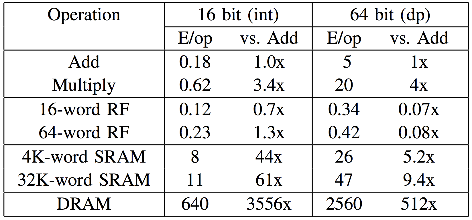
Figure 2. Memory access requires much more energy (640 pJ) than addition or multiplication.
Accessing cache memory (8 pJ) is much cheaper than using the main memory (table courtesy of Ardavan Pedram)
In order to get insight into how intrinsics instructions are implemented in Tensorflow Lite, we had to analyze some implementations including depthwise separable convolution with 3x3 kernels
Below we describe some of the main optimization techniques that are used for building lightweight and faster programs.
Loop Unrolling
Can you spot the difference between the following two code fragments?
for (int i = 0; i < 32; i++) {
  x[i] = 1;
  if (i%4 == 3) x[i] = 3;
}
for (int i = 0; i < 8; i++) {
  x[4*i  ] = 1;
  x[4*i+1] = 1;
  x[4*i+2] = 1;
  x[4*i+3] = 3;
}
The former way is what we usually write, and the latter is loop-unrolled version of former one.
Even though unrolling loops are discouraged from the perspective of software design and development due to severe redundancy, with low-level architecture this kind of unrolling has non-negligible benefits.
In the example described above, the unrolled version avoids examining 24 conditional statements in for loop, along with neglecting 32 conditional statements of if.
Furthermore, with careful implementation, these advantages can be magnified with the aid of SIMD architecture. Nowadays some compilers have options which automatically unroll some repetitive statements, yet they are unable to deal with complex loops.
Separate implementation for each case
Convolution layer can take several parameters.
For example, in depthwise separable layer, we can have many combinations with different parameters (depth_multiplier x stride x rate x kernel_size).
Rather than writing single program available to deal with every case, in low-level architectures, writing number of case-specific implementations is preferred.
The main rationale is that we need to fully utilize the special properties for each case.
For convolution operation, naive implementation with several for loops can deal with arbitrary kernel size and strides, however this kind of implementation might be slow.
Instead, one can concentrate on small set of actually used cases (e.g. 1x1 convolution with stride 1, 3x3 convolution with stride 2 and others) and fully consider the structure of every subproblem.
For example, in TensorFlow Lite there is a kernel-optimized implementation of depthwise convolution, targeted at 3x3 kernel size:
template <int kFixedOutputY, int kFixedOutputX, int kFixedStrideWidth, int kFixedStrideHeight>
struct ConvKernel3x3FilterDepth8 {};
Tensorflow Lite further specifies following 16 cases with different strides, width and height of outputs for its internal implementation:
template <> struct ConvKernel3x3FilterDepth8<8, 8, 1, 1> { ... }
template <> struct ConvKernel3x3FilterDepth8<4, 4, 1, 1> { ... }
template <> struct ConvKernel3x3FilterDepth8<4, 2, 1, 1> { ... }
template <> struct ConvKernel3x3FilterDepth8<4, 1, 1, 1> { ... }
template <> struct ConvKernel3x3FilterDepth8<2, 2, 1, 1> { ... }
template <> struct ConvKernel3x3FilterDepth8<2, 4, 1, 1> { ... }
template <> struct ConvKernel3x3FilterDepth8<1, 4, 1, 1> { ... }
template <> struct ConvKernel3x3FilterDepth8<2, 1, 1, 1> { ... }
template <> struct ConvKernel3x3FilterDepth8<4, 2, 2, 2> { ... }
template <> struct ConvKernel3x3FilterDepth8<4, 4, 2, 2> { ... }
template <> struct ConvKernel3x3FilterDepth8<4, 1, 2, 2> { ... }
template <> struct ConvKernel3x3FilterDepth8<2, 2, 2, 2> { ... }
template <> struct ConvKernel3x3FilterDepth8<2, 4, 2, 2> { ... }
template <> struct ConvKernel3x3FilterDepth8<2, 1, 2, 2> { ... }
template <> struct ConvKernel3x3FilterDepth8<1, 2, 2, 2> { ... }
template <> struct ConvKernel3x3FilterDepth8<1, 4, 2, 2> { ... }
Smart Memory Access Pattern
Since low-level programs are executed many times in repetitive fashion, minimizing duplicated memory access for both input and output is necessary. If we use SIMD architecture, we can load nearby elements together at once (Data Parallelism) and in order to reduce duplicated read memory access, we can traverse the input array by means of a snake-path.
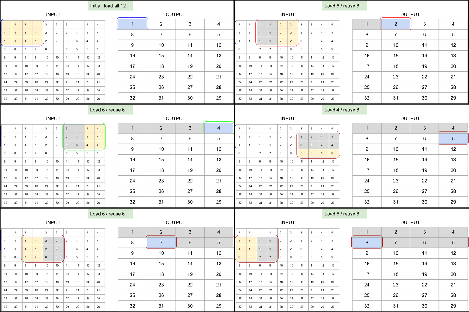
Figure 3. Memory access pattern for 8x8 output and unit stride, implemented in Tensorflow Lite's depthwise 3x3 convolution.
The next example which is targeted to be used in much smaller 4x1 output block also demonstrates how to reuse preloaded variables efficiently. Note that the stored location does not change for variables which are loaded in previous stage (in the following figure, bold variables are reused):
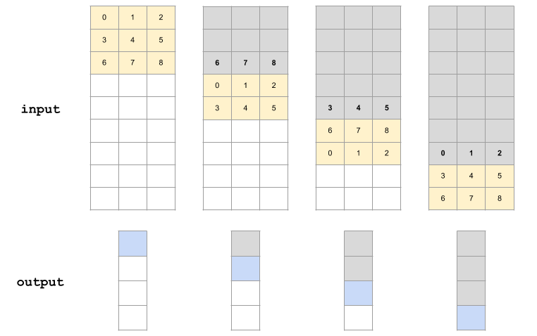
Figure 4. Memory access pattern for 4x1 output and stride 2, implemented in Tensorflow Lite's depthwise 3x3 convolution.
2) Be aware of using atrous depthwise convolution
Atrous (dilated) convolution is known to be useful to achieve better result for image segmentation[1]. We also decided to use atrous depthwise convolution in our network. One day, we tried to set stride for atrous depthwise convolution to make it accelerate computation, however we failed, because the layer usage in TensorFlow (≤ 1.8) is constrained.
In Tensorflow documentation of tf.nn.depthwise_conv2d (slim.depthwise_conv2d also wraps this function), you can find this explanation of rate parameter.
rate: 1-D of size 2. The dilation rate in which we sample input values across the height and width dimensions in atrous convolution. If it is greater than 1, then all values of strides must be 1.
Even though TensorFlow doesn’t support strided atrous function, it doesn’t raise any error if you set rate > 1 and stride > 1.
>>> import tensorflow as tf
>>> tf.enable_eager_execution()
>>> input_tensor = tf.constant(list(range(64)), shape=[1, 8, 8, 1], dtype=tf.float32)
>>> filter_tensor = tf.constant(list(range(1, 10)), shape=[3, 3, 1, 1], dtype=tf.float32)
>>> print(tf.nn.depthwise_conv2d(input_tensor, filter_tensor,
                                 strides=[1, 2, 2, 1], padding="VALID", rate=[2, 2]))

tf.Tensor(
[[[[ 302.] [ 330.] [ 548.] [ 587.]]
  [[ 526.] [ 554.] [ 860.] [ 899.]]
  [[1284.] [1317.] [1920.] [1965.]]
  [[1548.] [1581.] [2280.] [2325.]]]], shape=(1, 4, 4, 1), dtype=float32)

>>> 0 * 5 + 2 * 6 + 16 * 8 + 9 * 18   # The value in (0, 0) is correct
302
>>> 0 * 4 + 2 * 5 + 4 * 6 + 16 * 7 + 18 * 8 + 20 * 9   # But, the value in (0, 1) is wrong!
470
Let’s find the reason why this difference happened.
If we just put tf.space_to_batch and tf.batch_to_space before and after convolution layer, then we can use convolution operation for atrous convolution (profit!).
On the other hand, it isn’t straightforward how to handle stride and dilation together.
In TensorFlow, we need to be aware of this problem in depthwise convolution.
3) Architecture design principles for efficient segmentation network
Usually segmentation takes more time than classification since it has to upsample high spatial resolution map. Therefore, it is important to reduce inference time as much as possible to make the application run in real-time.
It is important to focus on spatial resolution when designing real-time application. One of the easiest ways is to reduce the size of input images without losing accuracy. Assuming that the network is fully convolutional, you can accelerate the model about four times faster if the size of input is halved. In literature[2], it is known that small size of input images doesn’t hurt accuracy a lot.
Another simple strategy to adopt is early downsampling when stacking convolution layers. Even with the same number of convolution layers, you can reduce the time with strided convolution or pooling within early layers.
There is also a tip for selecting the size of input image when you use Tensorflow Lite quantized model. The optimized implementations of convolution run best when the width and height of image is multiple of 8. Tensorflow Lite first loads multiples of 8, then multiples of 4, 2 and 1 respectively. Therefore, it is the best to keep the size of every input of layer as a multiple of 8.
Substituting multiple operations into single operation can improve speed a bit. For example, convolution followed by max pooling can be usually replaced by strided convolution. Transpose convolution can also be replaced by resizing followed by convolution. In general, these operations are substitutable because they perform the same role in the network. There are no big empirical differences among these operations.
Tips described above help to accelerate inference speed but they can also hurt accuracy. Therefore, we adopted some state-of-the-art blocks rather than using naive convolution blocks.
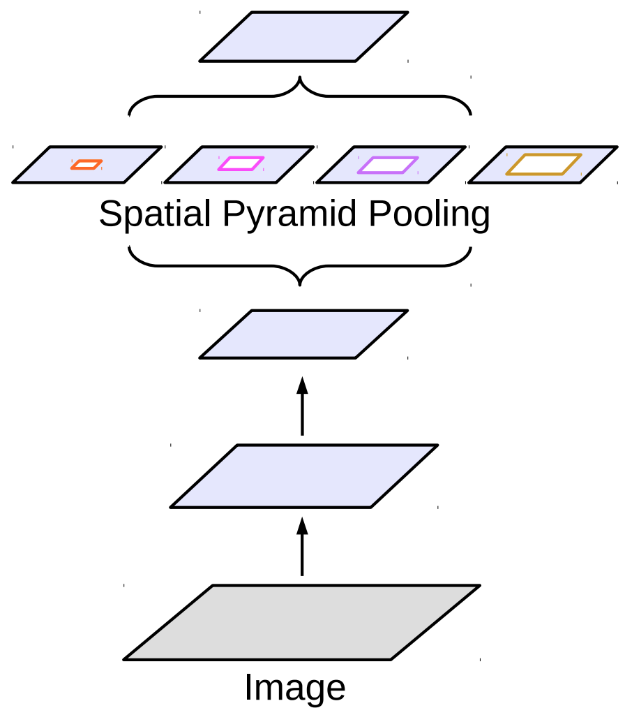
Figure 5. Atrous spatial pyramid pooling (figure courtesy of Liang-Chieh Chen)
Atrous spatial pyramid pooling[1] is a block which mimics the pyramid pooling operation with atrous convolution. DeepLab uses this block in the last layer.
We also substitute most of the convolution layers with efficient depthwise separable convolution layers. They are basic building blocks for MobileNetV1[3] and MobileNetV2[4] which are well optimized in Tensorflow Lite.
4) Folding batchnorm into atrous depthwise convolution
When quantizing convolution operation followed by batchnorm, batchnorm layer must be folded into the convolution layers to reduce computation cost. After folding, the batchnorm is reduced to folded weights and folded biases and the batchnorm-folded convolution will be computed in one convolution layer in TensorFlow Lite[5]. Batchnorm gets automatically folded using tf.contrib.quantize if the batchnorm layer comes right after the convolution layer. However, folding batchnorm into atrous depthwise convolution is not easy.
In TensorFlow’s slim.separable_convolution2d, atrous depthwise convolution is implemented by adding SpaceToBatchND and BatchToSpaceND operations to normal depthwise convolution as mentioned previously.
If you add a batchnorm to this operation by including argument normalizer_fn=slim.batch_norm, batchnorm does not get attached directly to the convolution layer.
Instead, the graph will look like the diagram below:
SpaceToBatchND → DepthwiseConv2dNative → BatchToSpaceND → BatchNorm
The first thing we tried was to modify TensorFlow quantization to fold batchnorm bypassing BatchToSpaceND without changing the order of operations.
With this approach, the folded bias term remained after BatchToSpaceND, away from the convolution layer.
Then, it became separate BroadcastAdd operation in TensorFlow Lite model rather than fused into convolution.
Surprisingly, it turned out that BroadcastAdd was much slower than the corresponding convolution operation in our experiment:
Timing log from the experiment on Galaxy S8
...
[DepthwiseConv] elapsed time: 34us
[BroadcastAdd]  elapsed time: 107us
...
To remove BroadcastAdd layer, we decided to change the network itself instead of fixing TensorFlow quantization.
Within slim.separable_convolution2d layer, we swapped positions of BatchNorm and BatchToSpaceND.
SpaceToBatchND → DepthwiseConv2dNative → BatchNorm → BatchToSpaceND
Even though batchnorm relocation could lead to different outputs values compared to the original, we did not notice any degradation in segmentation quality.
5) SIMD-optimized implementation for quantized resize bilinear layer
At the time of accelerating TensorFlow Lite framework, conv2d_transpose layer was not supported.
However, we could use ResizeBilinear layer for upsampling as well.
The only problem of this layer is that there is no quantized implementation, therefore we implemented our own SIMD quantized version of 2x2 upsampling ResizeBilinear layer.
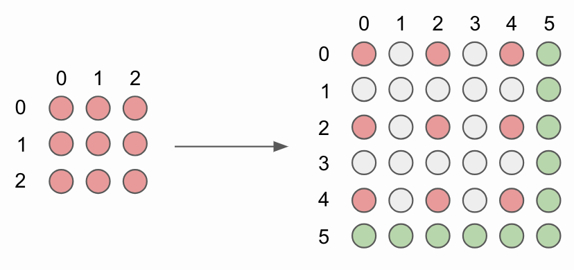
Figure 6. 2x2 bilinear upsampling without corner alignnment.
To upsample image, original image pixels (red circles) are interlayed with new interpolated image pixels (grey circles). In order to simplify implementation we do not compute pixel values for the bottommost and rightmost pixels, denoted as green circles.
for (int b = 0; b < batches; b++) {
  for (int y0 = 0, y = 0; y <= output_height - 2; y += 2, y0++) {
    for (int x0 = 0, x = 0; x <= output_width - 2; x += 2, x0++) {
      int32 x1 = std::min(x0 + 1, input_width - 1);
      int32 y1 = std::min(y0 + 1, input_height - 1);
      ResizeBilinearKernel2x2(x0, x1, y0, y1, x, y, depth, b, input_data, input_dims, output_data, output_dims);
    }
  }
}
Every new pixel value is computed for each batch separately.
Our core function ResizeBilinearKernel2x2 computes 4 pixel values across multiple channels at once.

Figure 7. Example of 2x2 bilinear upsampling of top left corner of image. (a) Original pixel values are simply reused and (b) – (d) used to interpolate new pixel values. Red circles represent original pixel values. Blue circles are new interpolated pixel values computed from pixel values denoted as circles with black circumference.
NEON (Advanced SIMD) intrinsics enable us to process multiple data at once with a single instruction, in other words processing multiple data at once.
Since we deal with uint8 input values we can store our data in one of the following formats uint8x16_t, uint8x8_t and uint8_t, that can hold 16, 8 and 1 uint8 values respectively.
This representation allows to interpolate pixel values across multiple channels at once.
Network architecture is highly rewarded when channels of feature maps are multiples of 16 or 8:
// Handle 16 input channels at once
int step = 16;
for (int ic16 = ic; ic16 <= depth - step; ic16 += step) {
  ...
  ic += step;
}

// Handle 8 input channels at a once
step = 8;
for (int ic8 = ic; ic8 <= depth - step; ic8 += step) {
  ...
  ic += step;
}

// Handle one input channel at once
for (int ic1 = ic; ic1 < depth; ic1++) {
  ...
}
SIMD implementation of quantized bilinear upsampling is straightforward. Top left pixel value is reused (Fig. 7a). Bottom left (Fig. 7b) and top right (Fig. 7c) pixel values are mean of two adjacent original pixel values. Finally, botom right pixel (Fig. 7d) is mean of 4 diagonally adjacent original pixel values.
The only issue that we have to take care of is 8-bit integer overflow.
Without a solid knowledge of NEON intrinsics we could go down the rabbit hole of taking care of overflowing by ourself.
Fortunately, the range of NEON intrinsics is broad and we can utilize those intrinsics that fit our needs.
The snippet of code below (using vrhaddq_u8) shows an interpolation (Fig. 7d) of 16 pixel values at once for bottom right pixel value:
// Bottom right
output_ptr += output_x_offset;
uint8x16_t left_interpolation = vrhaddq_u8(x0y0, x0y1);
uint8x16_t right_interpolation = vrhaddq_u8(x1y0, x1y1);
uint8x16_t bottom_right_interpolation = vrhaddq_u8(left_interpolation, right_interpolation);
vst1q_u8(output_ptr, bottom_right_interpolation);
6) Pitfalls in softmax layer and demo code
The first impression of inference in TensorFlow Lite was very slow. It took 85 ms in Galaxy J7 at that time. We tested the first prototype of TensorFlow Lite demo app by just changing the output size from 1,001 to 51,200 (= 160x160x2)
After profiling, we found out that there were two unbelievable bottlenecks in implementation.
Out of 85 ms of inference time, tensors[idx].copyTo(outputs.get(idx)); line in Tensor.java took up to 11 ms (13 %) and softmax layer 23 ms (27 %).
If we would be able to accelerate those operations, we could reduce almost 40 % of the total inference time!
First, we looked at the demo code and identified
tensors[idx].copyTo(outputs.get(idx)); as a source of problem.
It seemed that the slowdown was caused by copyTo operation, but to our surprise it came from int[] dstShape = NativeInterpreterWrapper.shapeOf(dst); because it checks every element (in our case, 51,200) of array to fill the shape.
After fixing the output size, we gained 13 % speedup in inference time.
<T> T copyTo(T dst) {
  ...
  // This is just example, of course, hardcoding output shape here is a bad practice
  // In our actual app, we build our own JNI interface with just using c++ code
  // int[] dstShape = NativeInterpreterWrapper.shapeOf(dst);
  int[] dstShape = {1, width*height*channel};
  ...
}
The softmax layer was our next problem.
TensorFlow Lite’s optimized softmax implementation assumes that depth (= channel) is bigger than outer_size (= height x width).
In classification task, the usual output looks like [1, 1(height), 1(width), 1001(depth)], but in our segmentation task, depth is 2 and outer_size is multiple of height and width (outer_size » depth).
Implementation of softmax layer in Tensorflow Lite is optimized for classification task and therefore loops over depth instead of outer_size.
This leads to unacceptably slow inference time of softmax layer when used in segmentation network.
We can solve this problem in many different ways. First, we can just use sigmoid layer instead of softmax in 2-class portrait segmentation. TensorFlow Lite has very well optimized sigmoid layer.
Secondly, we could write SIMD optimized code and loop over depth instead of outer_size.
You can see similar implementation at Tencent’s ncnn softmax layer, however, this approach has still its shortcomings.
Unlike ncnn, TensorFlow Lite uses NHWC as a default tensor format:

Figure 8. NHWC vs NCHW
In other words, for NHWC, near elements of tensor hold channel-wise information and not spatial-wise.
It is not simple to write optimized code for any channel size, unless you include transpose operation before and after softmax layer.
In our case, we tried to implement softmax layer assumming 2-channel output.
Thirdly, we can implement softmax layer using pre-calculated lookup table. Because we use 8-bit quantization and 2-class output (foreground and background) there are only 65,536 (= 256x256) different combinations of quantized input values that can be stored in lookup table:
for (int fg = 0; fg < 256; fg++) {
  for (int bg = 0; bg < 256; bg++) {
    // Dequantize
    float fg_real = input->params.scale * (fg - input->params.zero_point);
    float bg_real = input->params.scale * (bg - input->params.zero_point);

    // Pre-calculating Softmax Values
    ...

    // Quantize
    precalculated_softmax[x][y] = static_cast<uint8_t>(clamped);
  }
}
Conclusion
In this post, we described the main challenges we had to solve in order to run portrait segmentation network on mobile devices. Our main focus was to keep high segmentation accuracy while being able to support even old devices, such as Samsung Galaxy J7. We wish our tips and tricks can give a better understanding of how to overcome common challenges when designing neural networks and inference engines for mobile devices.
At the top of this post you can see portrait segmentation effect that is now available in Azar app. If you have any questions or want to discuss anything related to segmentation task, contact us at ml-contact@hcpnt.com. Enjoy Azar and mobile deep learning world!
References
[1] L. Chen, G. Papandreou, F. Schroff, H. Adam. Rethinking Atrous Convolution for Semantic Image Segmentation. June 17, 2017, https://arxiv.org/abs/1706.05587
[2] C. Szegedy, V. Vanhoucke, S. Ioffe, J. Shlens, Z. Wojna. Rethinking the Inception Architecture for Computer Vision. December 11, 2015, https://arxiv.org/abs/1512.00567
[3] A. Howard, M. Zhu, B. Chen, D. Kalenichenko, W. Wang, T. Weyand, M. Andreetto, H. Adam. MobileNets: Efficient Convolutional Neural Networks for Mobile Vision Applications, April 17, 2017, https://arxiv.org/abs/1704.04861
[4] M. Sandler, A. Howard, M. Zhu, A. Zhmoginov, L. Chen. MobileNetV2: Inverted Residuals and Linear Bottlenecks. January 18, 2018, https://arxiv.org/abs/1801.04381
[5] B. Jacob, S. Kligys, B. Chen, M. Zhu, M. Tang, A. Howard, H. Adam, D. Kalenichenko. Quantization and Training of Neural Networks for Efficient Integer-Arithmetic-Only Inference. December 15, 2017, https://arxiv.org/abs/1712.05877
Read more
-
Low Power Image Recognition Challenge 2018
Mobile Deep Learning approach to solving LPIRC 2018 challenge leading to the second place.