Disentangling Label Distribution for Long-tailed Visual Recognition

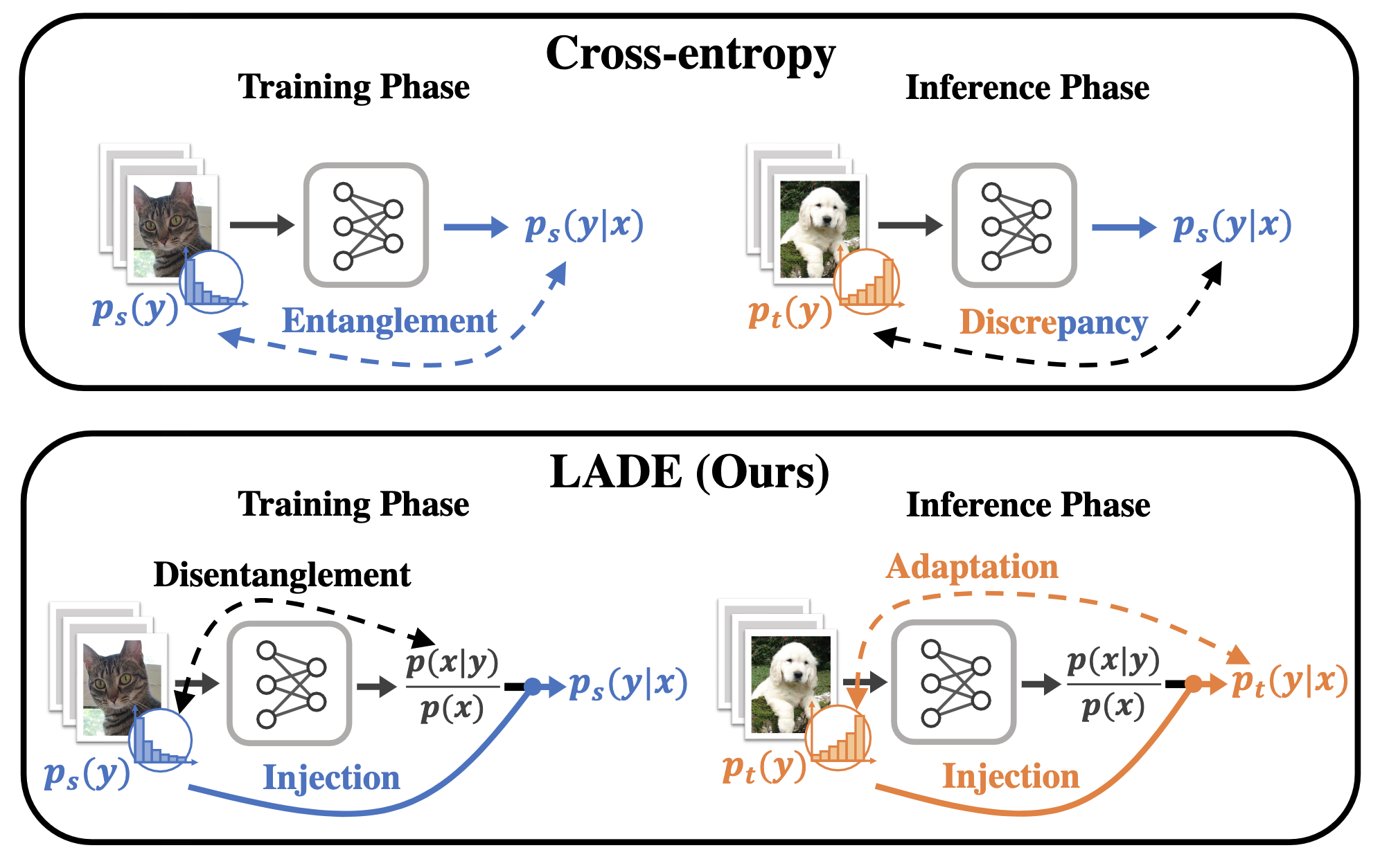
Unlike the vanilla cross-entropy loss for classification, our LADE loss disentangles the label distribution in training time - more details below.

We are happy to announce that our paper, “Disentangling Label Distribution for Long-tailed Visual Recognition” has been accepted to CVPR 2021!

What happens in real-world image classification tasks?

A machine learning engineer’s life would be much easier if every problem were like MNIST - training data being perfectly balanced and the test data distribution being identical to the training data. However, that’s never the case for real-world problems where data is often highly skewed. To make matters worse, we cannot escape from the fact that the trained model will encounter different situations than training after deployment. This paper primarily concentrates on two major issues: (1) Highly imbalanced training data and (2) Different train/test label distribution.

A slight hint of Bayesian scent

When we solve an image classification problem, we focus on two variables: input image \(x\) and output class label \(y\). Model’s concern is to estimate \(p(y|x)\), where it means “the probability of being the label \(y\) when the image \(x\) is given.” Using the Bayes rule, we can dissect \(p(y|x) = p(y) p(x|y) / p(x)\). Let’s dive deep into each of the components.

Deep dive: Label distribution \(p(y)\)

The easiest of the bunch is \(p(y)\): the label distribution. It’s simply the ratio of the labels in the data, which we can derive from the training data. \(p(y)\) for the test data is quite harder, but we assumed that we could estimate it in a feasible enough way. We can randomly sample some of the samples after deployment - we were already accumulating labels from time to time to evaluate running models anyways. Moreover, previous long-tailed literature usually doesn’t care about this issue - many of them assume the uniform distribution. It’s not that the others’ evaluation methods are problematic, as it’s an excellent way to evaluate all the classes fairly. We are just stating that it can be somewhat unrealistic in real-world settings, where test label distributions may vary significantly.

Aligning the label distribution by compensation

It turns out that there is already a simple but frequently ignored solution to this misalignment problem between the train and test label distribution. By simply dividing the trained \(p(y|x)\) with the training label distribution \(p_s(y)\) and multiplying with the test label distribution \(p_t(y)\), we can switch over the label distribution component of the \(p(y|x)\). We call this the Post-Compensation strategy (PC Strategy) in the paper and show its outstanding performance albeit its simplicity. But we didn’t stop here: can we fundamentally disentangle the label distribution from the trained model?

Deep dive: Image distribution \(p(x)\)

Before getting into our method, let’s briefly review the Bayes rule a bit further. It’s a bit more difficult to conceptualize the image distribution \(p(x)\). Let’s think of it this way: if we randomly painted a 224x224 image, it’ll end up with weird noises. However, suppose we did that enough number of times. In that case, a normal-ish image, or maybe the exact copy of the training image, may appear. The image distribution can be understood as a normal-ish-ness of the random image \(x\). \(p(x|y)\) is when you give label information too. An image of a car would not be appropriate for a cat image, right? However, it’s pretty hard to estimate both \(p(x)\) and \(p(x|y)\) directly, even if there are some recent attempts for it.

LADE loss directly regularizes the model output logits to be disentangled to the label distribution.

Donsker-Varadhan representation to the rescue

We shifted our views a little bit: how about estimating the likelihood ratio between the two: \(p(x|y) / p(x)\)? Luckily, there was already previous literature prepared for it: “Regularized Mutual Information Neural Estimation”. This paper concentrates on finding the mutual information between two distributions, where the loss function (the modified Donsker-Varadhan representation) yields the log-likelihood ratio of two arbitrary distributions. We simply plugged in the loss function as a regularizer for the standard cross-entropy loss and call this loss LAbel distribution DisEntangling (LADE) loss.

Performance evaluation

We evaluated both LADE and PC Strategy to the standard datasets that many long-tailed methods use: CIFAR-100-LT, Places-LT, ImageNet-LT, and iNaturalist 2018. LADE shows superior performances for all of the datasets, while PC Strategy often takes second place. Furthermore, we modified the standard test dataset to demonstrate different test label distribution settings (Variously shifted test label distributions). LADE shows excellent performance here also.

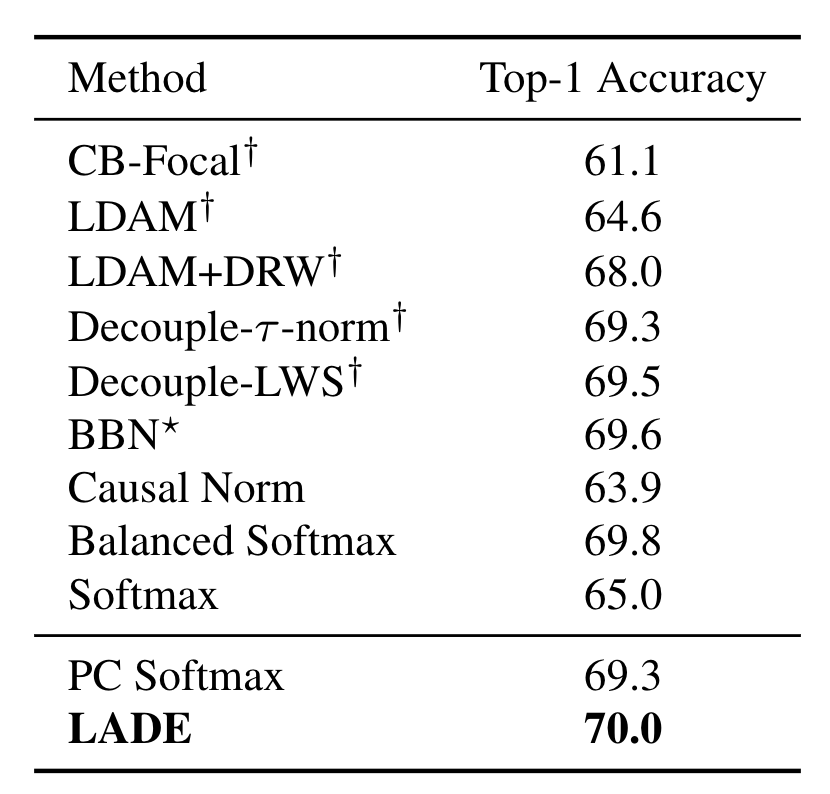Top-1 accuracy over all classes on iNaturalist 2018. LADE reaches the best accuracy among other methods, even without changing any network structure or a training scheme.

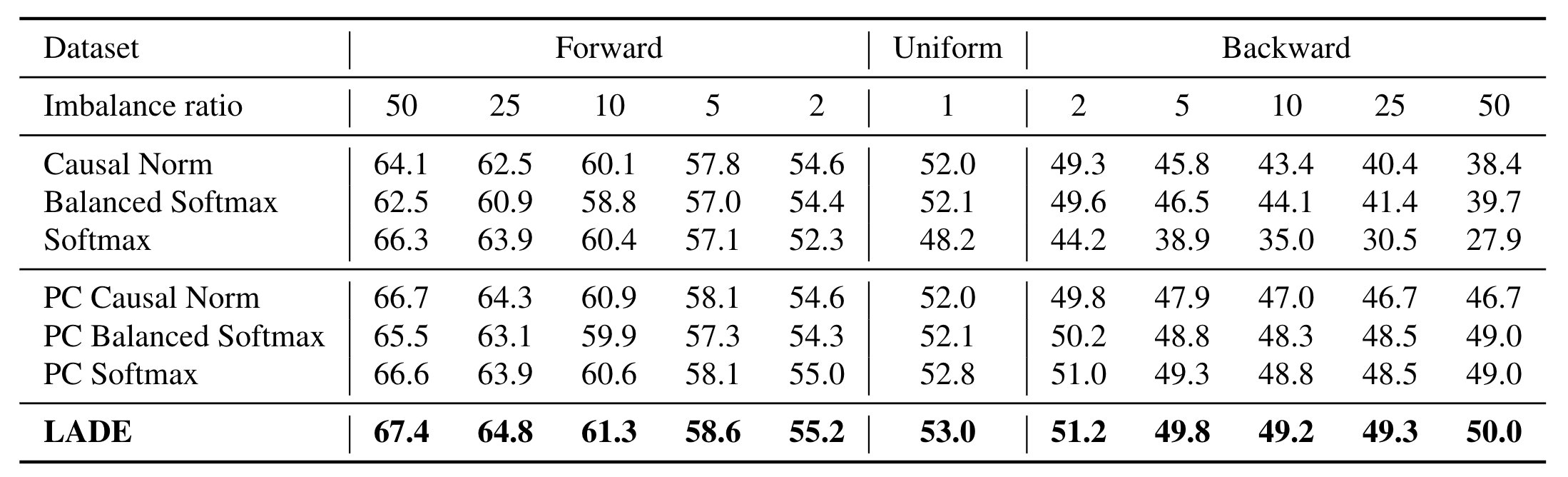Top-1 accuracy over all classes on test time shifted ImageNet-LT. PC strategy shows consistent performance gain, which indicates the benefits of plug-and-play target label distributions. Moreover, LADE outperforms all the other methods in every imbalance settings, and the performance gap between LADE and PC Softmax gets wider as the dataset gets more imbalanced.

Summary

We borrow the concept of label shift problem to suggest a more practical setting for the long-tailed visual recognition problem. To solve the problem, we design a novel loss that directly disentangles the label distribution from the trained model. Our method outperforms state-of-the-art long-tailed methods in various settings.